About Box Plus/Minus (BPM)
Box Plus/Minus, Version 2.0 (BPM) is a basketball box score-based metric that estimates a basketball player’s contribution to the team when that player is on the court. It is based only on the information in the traditional basketball box score--no play-by-play data or non-traditional box score data (like dunks or deflections) are included.
BPM uses a player’s box score information, position, and the team’s overall performance to estimate the player’s contribution in points above league average per 100 possessions played. BPM does not take into account playing time -- it is purely a rate stat! Playing time is included in Value Over Replacement Player (VORP) which is discussed below.
League average is defined as 0.0, meaning 0 points above average or below average. Because above-average players play more minutes, there are far more below-average players than above-average players in the league at any time. A value of +5.0 means the team is 5 points per 100 possessions better with the player on the floor than with average production from another player. (In the 2018-19 season, teams averaged around 100 possessions per 48 minute game.)
To give a sense of the scale:
- +10.0 is an all-time season (think peak Jordan or LeBron)
- +8.0 is an MVP season (think peak Dirk or peak Shaq)
- +6.0 is an all-NBA season
- +4.0 is in all-star consideration
- +2.0 is a good starter
- +0.0 is a decent starter or solid 6th man
- -2.0 is a bench player (this is also defined as "replacement level")
- Below -2.0 are many end-of-bench players
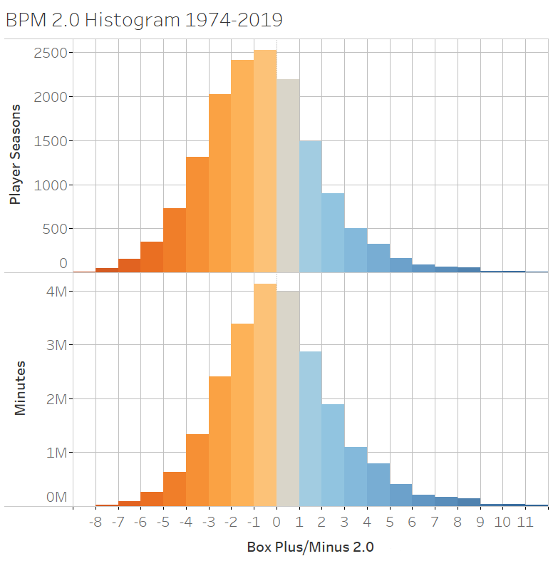
Here is a histogram of all player seasons from 1974 to 2019. Note that, by count of player seasons, there are far more below average seasons but that when you look at minutes played it is balanced.
For team scale, an elite team might have a regular-season team-level efficiency in the range of +8.0 per 100 team possessions. That elite team's best lineup of their five top players might be in the +14 range or even higher.
How does Box Plus/Minus evaluate players? The basic concept is simple. BPM starts by assuming that every player on the team has contributed equally. If the team is good, all of the players are assumed to be equally good.
Next, the box score information is added to revise the evaluation. All of the box score data is measured relative to the other players on the team. Does this player get more or fewer steals than the other players on the team? If more, this player is likely better on defense than they are. Do they score more or less efficiently? Do they have more or fewer assists?
This box score information is also weighted according to what position or role the player has on the team. For instance, a block by a center is good, but a block by a guard is great. Similarly, scoring by a low usage player has to be very efficient to mean much to the team, since they aren't putting pressure on the defense.
Now, some of the box score data does not help measure a player's impact on the team, even though the stat may be obviously valuable to the team. Defensive rebounds fall into that category. They matter to the team, but it really doesn't matter who on the team gets them. The credit for getting that rebound mostly gets split among the team, rather than all being credited to the player who actually pulled the rebound down.
BPM was created to intentionally only use statistics that are widely available and are available historically. Recently in the NBA far more statistics have been gathered, either from play-by-play or hand tracking, which allow more detailed metrics. BPM does not include that data and should not be as accurate as stats that do include the additional information (assuming they are implemented rigorously!) like Player Impact Plus/Minus and Real Plus/Minus.
There are limitations on all box score stats – if the box score doesn't measure a particular contribution, a box-score-based metric can only approximate that contribution. This is not a great hindrance on the offensive side, as nearly everything of importance on offense is captured by the box score (only missing things like screen-setting), but on defense the box score is quite limited. Blocks, steals, and rebounds, along with what little information offensive numbers yield about defensive performance are all that is available. Such critical components of defense as positioning, communication, and the other factors that make Kevin Garnett and Tim Duncan elite on defense can't be captured, unfortunately.
What does this mean? Box Plus/Minus is good at measuring offense and solid overall, but the defensive numbers in particular should not be considered definitive. Look at the defensive values as a guide, but don't hesitate to discount them when a player is well known as a good or bad defender.
Coverage
- From the 1985 season to the present, the BPM values presented are summed-up game level values. Summing up the game-level calculations better handles strength of schedule. This improvement mostly has an impact on players that missed a significant number of games.
- From 1974 through the 1984 season, the BPM values presented are the season-level values. From 1974 to 1977, turnovers are estimated using an approach given in the appendix.
How BPM is Calculated
Data Required
The following data is needed to calculate BPM:
- Player box score statistics per 100 possessions. (For instance this Team Per 100 Poss table.)
- Team Adjusted Efficiency per 100 possessions. (For instance the Team Rating table.)
- Player positions. Position and offensive role are estimated from box score data, unless the player has very few minutes.
Sequence of Calculation
- Calculate the player’s estimated position and offensive role, using the entire season’s worth of data. The full method for doing this is found in the Appendix below.
- Based on their position and role estimates, generate the player’s coefficients to be used in the raw BPM calculation. Some of the coefficients vary based on the player’s position and offensive role; some do not.
- Calculate the team-average points per adjusted shot attempt and compare this to the baseline points per adjusted shot attempt used by the regression.
- Adjust the points scored by the players on the team up or down by adding a constant points per adjusted shot attempt to all players on the team to account for this team shooting context.
- Calculate the raw BPM for the player.
- Sum up the raw BPM’s for the team (weighted by % of minutes played) and compare this to the team adjusted efficiency per 100 possessions.
- Add a constant (the "team adjustment") to the raw BPM of all of the players on the team so that the team's total sums to the team adjusted efficiency. Note--the team adjusted efficiency is corrected for the effect of leading or trailing.
- The player's raw BPM plus the team adjustment equals the completed BPM.
Follow along on the calculation with this Google Sheet: https://docs.google.com/spreadsheets/d/1PhD9eo3IqzpQo21-yVJPQzYjpXl_h-ZonIKqGEKBqwY/edit#gid=307166562
The Base Regression
The BPM 2.0 regression works off of per-100 possession statistics. All statistics are translated to per-100 team possessions. While this can potentially lose a bit of nuance (for instance, not accounting for the number of opportunities for the given stat to be accrued), it does streamline everything about the calculation. The output of the regression is in points per 100 team possessions.
As mentioned above: the coefficients vary by the position and offensive role the player plays. In other words, some statistics mean different things if the player plays point guard versus if the player is a center.
To do this, every player is assigned a standard position value and also an offensive "creation" position value. Both of these position spectrums vary between position 1 (PG & Creator) and position 5 (Center & Receiver). These position scales are calculated using regressions found in the appendix.
Here are the variables and coefficients used:
| Box Plus/Minus Regression | ||
| Coefficient | ||
| Variable | Position 1.0 (PG) | Position 5.0 (C) |
| Pts (adjusted for team context) | 0.860 | |
| 3PM (3 pointer made) | 0.389 | |
| AST | 0.580 | 1.034 |
| TO | -0.964 | |
| ORB | 0.613 | 0.181 |
| DRB | 0.116 | 0.181 |
| STL | 1.369 | 1.008 |
| BLK | 1.327 | 0.703 |
| PF | -0.367 | |
| Coefficient | ||
| Variable | Offensive Role 1.0 (Creator) | Offensive Role 5.0 (Receiver) |
| FGA | -0.560 | -0.780 |
| FTA (=0.44*FGA) | -0.246 | -0.343 |
The coefficients vary linearly between position 1 and position 5. If a player is position 1, the coefficients for position 1 in the table above are used. If a player is position 3 (i.e. small forward), then coefficients halfway between the first column and the second column are used, since position 3 is halfway between position 1 and position 5.
Discussing these values:
- Points are a constant value across positions.
- Field goal attempts are a higher "cost" for low-usage players--they are more frequently assisted and the values reflect this.
- The 3PM coefficient was set to be uniform across all positions. This bonus accounts for the value of spacing and any other ancillary benefits of shooting more 3s.
- Assists are worth far more for a post player than for a point guard. Point guards handle the ball a lot and usually generate lower value assists. A center’s assists are usually very high value. In addition, post players that pass well are typically better defenders.
- Rebounding is interesting. For bigs, a rebound is a rebound. For guards, offensive rebounds are worth quite a bit. Defensive rebounds by guards mean almost nothing in this regression (in other words, the credit is split perfectly evenly to all 5 players).
- Steals and blocks are both worth more for the little guy than for the post players.
- Personal fouls are a negative for both guards and bigs.
| Position Adjustment Constant | |||
| Position 1 (PG) | Position 3 (SF) | Position 5 (C) | |
| Position Constant | -0.818 | 0.00 | 0.00 |
In addition, there is a position adjustment constant that is not linear between positions 1 and 5. The value is 0 for positions above 3 (small forward), but drops linearly to a value of -0.818 at position 1. In other words, for all players with a position bigger than SF, there is no adjustment, but point guards get the biggest penalty. The justification for this is that PGs and to some extent SGs do not provide as much value that is not captured in the box score, mostly related to defense.
| Offensive Role Adjustment Constant | |||
| 1.0 (Creator) | 3.0 (Neutral) | 5.0 (Receiver) | |
| Position Constant | -2.774 | 0.00 | 2.774 |
Similarly, there is also an offensive role adjustment. Players who do not have a large offensive role are typically penalized by a box score analysis, so they have an upward adjustment as seen above.
Sample Raw GmBPM Calculation
Here’s a sample calculation for this part of the metric:
2017 LeBron James
The position regression estimates that he is position 2.3 (rather than the listed SF). His offensive role is 1.0 (pure creator).
| Variable | Coefficient | Per 100 Possession Statistics (2017 LeBron) | Total |
| Pts (adjusted for team context) | 0.860 | 34.9 adjusted to 30.4 | 26.1 |
| 3PM | 0.389 | 2.2 | 0.9 |
| AST | 0.727 | 11.5 | 8.4 |
| TO | -0.964 | 5.4 | -5.2 |
| ORB | 0.473 | 1.7 | 0.8 |
| DRB | 0.137 | 9.7 | 1.3 |
| STL | 1.252 | 1.6 | 2.0 |
| BLK | 1.125 | 0.8 | 0.9 |
| PF | -0.367 | 2.4 | -0.9 |
| FGA | -0.560 | 24.0 | -13.4 |
| FTA | -0.246 | 9.5 | -2.3 |
| TOTAL | 18.7 |
Then comes the position and offensive role constants. LeBron’s position is 2.3, so his position constant is (3-2.3)*(-0.818/2)=-0.3. His offensive role is 1.0, so his offensive role constant is (3.0-1.0)*(-2.774/2)= -2.8. Together, the constants total to -3.1. Thus LeBron’s overall Raw BPM in 2017 is 18.7 - 3.1 = 15.6.
Team Adjustment
Next comes the team adjustment, which, like the original BPM, is a CRITICAL part of the metric. The regression was generated with the team adjustment part of the fit. It allows the regression to assign credit to other players on the floor besides the player who actually posted the stat. This shows up most obviously in the value for rebounds--a defensive rebound is worth quite a bit to the team, but the individual value assigned above is small (or almost nothing, for point guards!) The unassigned remaining credit is split amongst all players that are on the floor.
The team adjustment is fairly simple. If a team is a +0.0 efficiency (in points per 100 possessions) team, then the adjusted GmBPM values, when weighted by % of possessions played, must sum to +0.0. A simple constant will be added to all of the Raw GmBPM values to make this sum properly. Please note--these team adjustment constants will generally be around -8. This is because this constant is also acting as the intercept for the regression.
Now, we do not actually sum to the team’s efficiency. Jeremias Englemann demonstrated that players play worse with the lead and better if behind. The effect is linear and has been consistently replicated. The team in the lead plays about 0.35 pts/100 possessions worse for every point of lead. To adjust for this, we must estimate what the team’s average lead was, and then add or subtract one half of the effect (the other half is assumed to belong to the opponents). There are a number of ways to estimate the lead (or actually calculate it). A quick estimate puts 2017 Cleveland at an average lead of around 1.4 points. The effect of playing with that lead is -0.35/2*1.4 = -0.24, which shifts the Team’s Adjusted Rating from +3.0 to +3.24.
Now, the actual calculation is done. The RawBPM * % of minutes played is summed across the team, then the constant is calculated to shift that total so it sums to the adjusted team rating (+3.24). For 2017 Cleveland, that team adjustment is -8.0.
So, LeBron’s 2017 Box Plus/Minus for the regular season comes in at 15.6 - 8.0 = +7.6 points per 100 possessions. That’s an elite number, but not quite up to his prior peaks.
The Regression Basis
One of the unique things about this analysis is the regression basis that was used. It is not a simple long-term Regularized Adjusted Plus/Minus (RAPM).
- Four 5-year long RAPM regressions (covering 1996-97 to 2015-16)
- Bayesian prior-informed, using a prior that is based only on team quality and minutes per game in the given season. This eliminates the need for an aging adjustment within the regression to handle year-to-year aging shifts.
- The prior also solves the issue of low-minutes players regressing towards league-average.
- Special thanks to James Brocato of the Dallas Mavericks for running this Bayesian RAPM specially for the development of this new version of BPM!
Since these are only 5-year-long sets, a smaller portion of a player’s career is captured, including higher highs and (to some extent) lower lows.
Here is a sample of the dataset. Yes, Steve Nash was ridiculous on offense, and no, the box score still can’t fully capture that fact.
The Offense/Defense Split
To split BPM into offensive and defensive components, the same style of regression is used. It outputs offensive BPM, and defensive BPM is simply calculated as Total BPM - Offensive BPM. The regression coefficients were developed to maximize the fit for both offense and defense concurrently.
The Offense/Defense regression uses the same variables as full BPM, just with different coefficients.
Here are the coefficients used:
| Offensive Box Plus/Minus Regression | ||
| Coefficient | ||
| Variable | Position 1.0 (PG) | Position 5.0 (C) |
| Pts (adjusted for team context) | 0.605 | |
| 3PM (3 pointer made) | 0.477 | |
| AST | 0.476 | |
| TO | -0.579 | -0.882 |
| ORB | 0.606 | 0.422 |
| DRB | -0.112 | 0.103 |
| STL | 0.177 | 0.294 |
| BLK | 0.725 | 0.097 |
| PF | -0.439 | |
| Coefficient | ||
| Variable | Offensive Role 1.0 (Creator) | Offensive Role 5.0 (Receiver) |
| FGA | -0.330 | -0.472 |
| FTA (=0.44*FGA) | -0.145 | -0.208 |
The coefficients vary linearly between position 1 and position 5. If a player is position 1, the coefficients for position 1 in the table above are used. If a player is position 3 (i.e. small forward), then coefficients halfway between the first column and the second column are used, since position 3 is halfway between position 1 and position 5.
Discussing these values:
- Points and field goal attempts for OBPM look similar to the full BPM regression.
- The 3 pt bonus is larger than for BPM. This indicates players shooting 3s are a large benefit on offense but a small hindrance to the defense.
- Assists are interesting. For guards, the BPM and OBPM coefficients are similar. For bigs, though, the offensive value of assists is less than the total value. Assists are a significant indicator of defensive skill for bigs.
- Offensive rebounds are worth more to the offense than overall, indicating they help the offensive quite a bit but hurt the defense a little.
- Blocks are interesting--they are a big positive indicator for a guard’s offense!
- Personal fouls are a large negative to the offensive value of a player but are a small positive to their defensive value.
| Position Adjustment Constant | |||
| Position 1 (PG) | Position 3 (SF) | Position 5 (C) | |
| Position Constant | -1.698 | 0.00 | 0.00 |
Like for the overall BPM, there is a position adjustment constant that is not linear between positions 1 and 5.
| Offensive Role Adjustment Constant | |||
| 1.0 (Creator) | 3.0 (Neutral) | 5.0 (Receiver) | |
| Position Constant | -0.860 | 0.00 | 0.860 |
Similarly, there is also an offensive role adjustment. The scale is much smaller for offensive BPM than overall, indicating that much of the value not captured in the box score is on defense (which makes sense.)
Doing this at the Game Level
This same analysis works at the game level, if box scores are available. On basketball reference, this approach is available back to 1985. Positions and offensive roles are still estimated at the season level, but the regression, including the adjustments, are run at the game level.
The team adjustment is a little more complex. What should the team sum to?
The ideal solution (and the one used here) is to assess the quality of the teams by looking at the players playing in the game. This accounts for players missing games or, in the playoffs, teams using shorter rotations. Add up all of the players’ regular season, season-level BPM ratings, weighted by % of possessions played in this game. This gives the overall quality of the game. Next, the efficiency margin of the game itself, adjusted by the average lead in the game, is added to the two team’s ratings.
For instance: in a playoff game, with shortened playoff lineups, the average team efficiency as estimated by the players’ regular season BPMs may be +10 for the two teams. If one team won by +12 efficiency differential, with an average lead of +5 points, the team’s ratings would be as follows:
- Winning team: +10 +12/2 +(0.35/2)*5 = +16.9 points
- Losing team: +10 -12/2 -(0.35/2)*5 = +3.1 points
This sounds relatively straightforward, but how does this work with players with very few minutes and outlier BPMs? A very simple regression to the mean was included to remove oddities. A projected BPM was developed in the following manner:
- Estimate a regressed minutes per game the player plays. This is done by taking the players minutes and dividing by the number of games they have played plus 4.
- Create an estimated BPM based on the regressed minutes played. This is calculated as - 4.75 + 0.175 * ReMPG.
- Create a minutes weight for this estimated BPM. It is (450 - Minutes)/3, with a minimum of 0. This creates a linear weight starting at 150 when the player has zero minutes and scaling down to zero when the player has 450 minutes.
- The regressed BPM value that will be used in the game-level team strength calculations is then the weighted average of the player's season-level BPM, weighted by minutes played, and the estimated BPM listed above, weighted by the minutes weight.
- These calculations were developed to stabilize low minutes players without significantly impacting higher minutes players. It has typically been the case that low minutes players are approximately equal in quality across all NBA teams, regardless of the team strength.
Alternatively, a similar calculation may be done simply using the two team’s adjusted efficiency differentials instead of looking at the actual quality of the players playing in the game. This approach would be computationally much easier but would lose the benefit of accounting for who was actually playing in the game and for how long. This approach is more appropriate when using NCAA college data, since the low minutes adjustment is more challenging.
Here is how BPM 2.0 Season level compares to BPM 2.0 Game level:
The fit is very close. Adding the more accurate game-level data does not have a huge impact but in individual cases can make a difference of 0.5 BPM or more, particularly when a player has only played a partial season with the team or missed a lot of games due to injury.
Looking at Results: The All-Time Great Seasons
To give a sense of the metric, it is useful to look at some of the great seasons. Here are the top 15 of all time by BPM, minimum 1000 minutes played:
| Rank | Player | Year | Team | BPM | OBPM | DBPM |
| 1 | LeBron James | 2009 | CLE | 13.2 | 9.5 | 3.7 |
| 2 | Michael Jordan | 1988 | CHI | 13.0 | 8.8 | 4.2 |
| 3 | Michael Jordan | 1991 | CHI | 12.0 | 8.9 | 3.2 |
| 4 | Stephen Curry | 2016 | GSW | 11.9 | 10.4 | 1.6 |
| 5 | Michael Jordan | 1989 | CHI | 11.9 | 8.4 | 3.4 |
| 6 | David Robinson | 1994 | SAS | 11.9 | 8.1 | 3.8 |
| 7 | LeBron James | 2010 | CLE | 11.8 | 9.1 | 2.8 |
| 8 | LeBron James | 2013 | MIA | 11.7 | 9.3 | 2.4 |
| 9 | Michael Jordan | 1993 | CHI | 11.2 | 8.7 | 2.6 |
| 10 | Michael Jordan | 1990 | CHI | 11.2 | 9.1 | 2.1 |
| 11 | Russell Westbrook | 2017 | OKC | 11.1 | 8.7 | 2.4 |
| 12 | Chris Paul | 2009 | NOH | 11.0 | 7.2 | 3.8 |
| 13 | James Harden | 2019 | HOU | 11.0 | 9.4 | 1.6 |
| 14 | LeBron James | 2012 | MIA | 10.9 | 8.2 | 2.7 |
| 15 | LeBron James | 2008 | CLE | 10.9 | 8.2 | 2.6 |
Notice that Russell Westbrook’s 2017, which in BPM 1.0 was +15.6 and the top of all time, dropped down significantly. Also notice that LeBron and Jordan dominate this list. Older players did not dominate the game the way newer players can, primarily due to rule changes.
All time offensive seasons:
| Rank | Player | Year | Team | OBPM |
| 1 | Stephen Curry | 2016 | GSW | 10.4 |
| 2 | Tracy McGrady | 2003 | ORL | 9.8 |
| 3 | LeBron James | 2009 | CLE | 9.5 |
| 4 | James Harden | 2019 | HOU | 9.4 |
| 5 | LeBron James | 2013 | MIA | 9.3 |
| 6 | Michael Jordan | 1990 | CHI | 9.1 |
| 7 | LeBron James | 2010 | CLE | 9.1 |
| 8 | Michael Jordan | 1991 | CHI | 8.9 |
| 9 | Michael Jordan | 1988 | CHI | 8.8 |
| 10 | Kevin Durant | 2014 | OKC | 8.8 |
And the all time defensive seasons:
| Rank | Player | Year | Team | DBPM |
| 1 | Nate McMillan | 1994 | SEA | 5.5 |
| 2 | Manute Bol | 1986 | WSB | 4.7 |
| 3 | David Robinson | 1992 | SAS | 4.6 |
| 4 | Manute Bol | 1987 | WSB | 4.6 |
| 5 | Manute Bol | 1988 | WSB | 4.5 |
| 6 | Mark Eaton | 1983 | UTA | 4.3 |
| 7 | Mark Eaton | 1985 | UTA | 4.2 |
| 8 | Randy Brown | 1995 | SAC | 4.2 |
| 9 | Michael Jordan | 1988 | CHI | 4.2 |
| 10 | Nate McMillan | 1996 | SEA | 4.2 |
Box Plus/Minus is a very good offensive metric, but it struggles some with defense. As mentioned before, when all you have is a box score, you cannot estimate defense very well. Not including minutes per game in the regression also hampers the accuracy of the defensive estimates. In other words--take DBPM with a spoonful of salt.
Looking at the Results: Charts
Another way to look at the results is with an interactive chart. This plots the base RAPM on the x axis and BPM 2.0 and BPM 1.0 on the y axis. Use the selection button at the top left to look at total BPM, offense only, or defense only.
History of Box Plus/Minus
In order to create a box-score-based player evaluation metric, some basis for the weights given to each statistic must be chosen. A number of different "box-score" stats have been developed over the years: some of the more intricate and well-known include John Hollinger's PER (further explanation at ESPN), Justin Kubatko's Win Shares here at Basketball Reference, and Dave Berri's Wins Produced.
The approach followed with Box Plus/Minus leans toward the empirical side, following the concepts of a "Statistical Plus/Minus (SPM)" metric. Please read Neil Paine's review of SPM at the Basketball Reference Blog to understand the background of this approach, originally pioneered by Dan Rosenbaum as a sideline to his Adjusted Plus/Minus (APM) work.
The original Box Plus/Minus was originally released on Basketball Reference in 2014 after several years of development. It used a very-long-term Regularized Adjusted Plus/Minus (RAPM) as its regression basis, used "advanced box score" metrics (i.e. rebounds per rebounding opportunity), and included a couple of nonlinear interaction terms between usage, rebounds, and assists.
It worked very well, but it did have some issues:
- Nonlinear terms. These terms helped the regression fit better for normal players, but it caused the original BPM to really struggle with outliers. Russell Westbrook’s 2017 MVP campaign made it clear!
- Narrow regression basis. A very-long-term Regularized Adjusted Plus/Minus was used as basis for developing the original BPM. This made the issues with capturing outliers significantly worse, as no player was elite or an outlier for the entire 14 years captured in the regression basis.
- Inclusion of Minutes-per-Game (MPG) in the regression. MPG will always help the statistic be more accurate overall--coaches generally know what they are doing. However, minutes allotment depends on a lot of factors beyond actual quality of play on the court. So while the overall fit improves with it included, it is also introducing another source of bias to the regression. Secondly, it overlaps with the information provided by the actual box score. This greatly complicates interpreting the value of actual actions on the court--the value of a steal is reflected both by MPG and the steal statistic itself. Finally, Box Plus/Minus 2.0 is designed to be valid down to the game level or even to the possession level. Obviously, MPG at the game level is just a single data point that could vary widely for a wide number of reasons and is not stable.
The new BPM was developed with these issues always in mind, with a goal of fully resolving the problems. It includes:
- Superior regression basis (much wider data spread, much larger overall dataset, much less biased).
- Fully linear regression (much more robust when faced with outlier data). This also can be used on much smaller data samples and still produce realistic results.
- No MPG in the regression. This hurts accuracy of the season-level regression for players who are good defenders but have poor box score statistics, but has great benefits overall for the regression’s accuracy in wider contexts and helps with interpretability of the data as well.
Similar Linear Box Score Metrics
Several other NBA statisticians have created truly linear statistical plus/minus metrics along similar lines. While BPM has differences, the end goals and general methodology owe a debt to them:
- Simple Player Rating (SPR) was developed by Nathan Walker (@bbstats) many years ago (2012) and was the first simplified linear metric built by regressing box score stats onto a long-term RAPM basis--in this case, an 8 year data set. He developed this shortly after I developed Advanced Statistical Plus/Minus (ASPM), the precursor to Box Plus/Minus. ASPM was fancier...but not always in a good way.
- Daily RAPM Estimator (DRE) was developed by Kevin Ferrigan (@NBAcouchside) and similarly regressed box score statistics onto a long-term RAPM estimate--here the 14-year average RAPM dataset created by Jeremias Engelmann (who also co-developed Real Plus/Minus). Given the good RAPM basis, this linear metric has probably become the most widely used for small-sample-size evaluations.
Value over Replacement Player
Value over Replacement Player (VORP) converts the BPM rate into an estimate of each player's overall contribution to the team, measured vs. what a theoretical "replacement player" would provide, where the "replacement player" is defined as a player on minimum salary or not a normal member of a team's rotation. A long and comprehensive discussion on defining this level for the NBA was had at Tom Tango's blog, and is worth a read. (Tom Tango is a baseball sabermetrics expert, and one of the originators of the replacement level framework and the Wins Above Replacement methodology common now in baseball.)
The conclusion was to establish -2.0 as replacement level for the NBA, measured in terms of points above or below average per 100 possessions.
Now, players will have BPMs below that -2.0 replacement level. In basketball, there can be several reasons why:
- The player is actually below replacement level skill. (Sometimes this is because they are young and developing).
- The player is not actually that bad, but is having bad shooting luck.
- The player is playing in a bad situation/context for them, where their good qualities are minimized and weaknesses exaggerated.
- The player is being developed (being asked to stretch their skills beyond their current skill level). This happens more often in the NBA than, for instance, in baseball.
- BPM is not capturing what a player contributes. This is particularly an issue for elite defenders where BPM simply does not recognize them from their box score statistics.
- If one were to define a "replacement level" for offense and defense, it would be -1.7 on offense and -0.3 on defense – though the concept of replacement level for components doesn't necessarily make sense. Almost all point guards would be well below the -0.3 level on defense, since a guard's role is primarily to focus on offense. The reverse is true of post players. It's an interesting exercise, but ultimately OVORP and DVORP aren't that useful, and will not be displayed here.
So, to calculate VORP, the formula is simply: [BPM - (-2.0)] * (% of possessions played) * (team games/82). This yields the number of points the player is producing over a replacement player, per 100 TEAM possessions over an entire season. This normalizes all of the players to the same pace environment, so if a team plays at a much faster pace, they in reality would have a much larger number of possessions and a larger average actual point differential, but this calculation looks per 100 possessions.
As an example: In 2017, LeBron had a BPM of +7.6, and he played 70% of Cleveland's minutes. His VORP, then, would be [7.6 – (-2.0)] * 0.70 * 82/82 = 6.7.
The beauty of VORP is that like WAR in baseball, it should track linearly with salary. A player with a VORP of 4.0 is worth, on the market, about twice what a player of VORP 2.0 is worth. Sometimes good players play only a few minutes for reasons outside their control, and would be worth more because they should be getting more minutes. Still, for a crude estimate, VORP is valuable. It measures reasonably accurately what a player did produce in terms of value for a given team.
To convert VORP to an estimate of wins over replacement, simply multiply by 2.7. This translates a player's efficiency differential approximately into wins, using the conversion rate near league-average rather than that in the diminishing returns area of the Pythagorean formula. By this methodology, Michael Jordan in 1989 was worth about 31 wins. (In reality, he would quickly push an average team into the diminishing returns region of the points-to-wins conversion.)
Here's a look at the top 15 seasons of all time by VORP. This is the best measure of actual value contributed to the team. Notice that Michael Jordan played a few more minutes per season than LeBron, thus increasing his overall value.
| Rank | Player | Year | Team | VORP | Minutes | BPM |
| 1 | Michael Jordan | 1988 | CHI | 12.5 | 3311 | 13.0 |
| 2 | LeBron James | 2009 | CLE | 11.8 | 3054 | 13.2 |
| 3 | Michael Jordan | 1989 | CHI | 11.4 | 3255 | 11.9 |
| 4 | David Robinson | 1994 | SAS | 11.4 | 3241 | 11.9 |
| 5 | Michael Jordan | 1991 | CHI | 10.8 | 3034 | 12.0 |
| 6 | Michael Jordan | 1990 | CHI | 10.7 | 3197 | 11.2 |
| 7 | Michael Jordan | 1987 | CHI | 10.6 | 3281 | 10.8 |
| 8 | LeBron James | 2010 | CLE | 10.4 | 2966 | 11.8 |
| 9 | Michael Jordan | 1993 | CHI | 10.3 | 3067 | 11.2 |
| 10 | LeBron James | 2013 | MIA | 10.0 | 2877 | 11.7 |
| 11 | Kevin Garnett | 2004 | MIN | 9.9 | 3231 | 10.2 |
| 12 | Chris Paul | 2009 | NOH | 9.9 | 3002 | 11.0 |
| 13 | LeBron James | 2008 | CLE | 9.8 | 3027 | 10.9 |
| 14 | Michael Jordan | 1996 | CHI | 9.8 | 3090 | 10.5 |
| 15 | Dwyane Wade | 2009 | MIA | 9.7 | 3048 | 10.6 |
Here is a chart of VORP vs. BPM:
Appendices:
Position and Offensive Role Regressions:
The position regression was developed by regressing player statistics on listed positions over a 20-year sample of player seasons, weighted by minutes played. This calculation works off of percentages of team statistics accrued by the player while they are in the game. Here are the coefficients:
| Current | Pre-1974 | |
| Intercept | 2.130 | 1.590 |
| % of Team TRB | 8.668 | 10.892 |
| % of Team STL | -2.486 | |
| % of Team PF | 0.992 | 1.468 |
| % of Team AST | -3.536 | -4.400 |
| % of Team BLK | 1.667 |
For small sample sizes, this regression may not produce valid results, so a weighted average of the results of this regression (weighted by minutes played) and 50 minutes of the player’s listed position is used. The regression output is then limited to a minimum of 1.0 and a maximum of 5.0.
Next, the team sum is calculated to make sure that the minutes-weighted team average is 3.0. A constant is added to the regression sum of each of the team’s players (prior to the 1.0 and 5.0 limitation) to shift the players on the team so that the sum equals 3.0. (This is done recursively because of the 1.0 and 5.0 limits for the players.)
When the position regression weights were developed, all of these steps were included in the model, so the regression weights are optimized for usage in this way.
The offensive role regression was developed differently. It was based on the past 15 years of assist, shooting location, and assisted percentage numbers from play-by-play data. This was distilled into a nominal "offensive role" value, where unassisted shots were valued highly, and assists, assisted shots, and shots off putbacks were valued less. Shooting efficiency was also included. This "offensive role" was then used as a regression basis for a simple regression again using % of team statistics.
The values found were:
| Coefficient | |
| Intercept | 6.00 |
| % of Team AST | -6.642 |
| % of Team Threshold Points | -8.544 |
"Threshold points" is calculated as points above a threshold Points/True Shot Attempt level, where the threshold shooting efficiency is 0.33 points below the team average Points/True Shot Attempt. This 0.33 point value was found as part of the regression.
Again, to assist with small sample sizes, an additional value of 50 minutes at an Offensive Role of 4.0 is added, and then the regression output is limited to a minimum of 1.0 and a maximum of 5.0.
Next, the team sum is calculated to make sure that the minutes-weighted team average is 3.0. A constant is added to the regression sum of each of the team’s players (prior to the 1.0 and 5.0 limitation) to shift the players on the team so that the sum equals 3.0. (This is done recursively because of the 1.0 and 5.0 limits for the players.)
Because the statistics used in estimating player position and offensive role do not overlap much, it is theoretically possible to have a position of 5.0 and a creation role of 1.0.
Imputed Turnover Estimator (1974-1977)
This uses Per 100 possession stats as inputs to estimate turnovers per 100 possessions:
| Intercept | Age | Year | PTS | TRB | FGA | FTA | AST | PF | |
| Coefficients | 4.1119 | -0.0191 | -0.0519 | -0.0494 | 0.0442 | 0.0957 | 0.2056 | 0.2216 | 0.1972 |
Year is here just the last 2 digits of the year (turnovers steadily dropped through the sample I reviewed). Note, this regression only is a correlation of 0.71 with actual turnovers...it's pretty tough to estimate closely. Turnovers don't really correlate with any other stat very closely. Still, it should be OK for the new BPM estimation. The average error is 0.5 TOV/100 possessions.
This produces TOV/100 poss. Average is around 3.7.

We're Social...for Statheads
Site Last Updated: Sunday, June 14, 7:41PM
Question, Comment, Feedback, or Correction?
Subscribe to our Free Email Newsletter
Subscribe to Stathead Basketball: Get your first month FREE
Your All-Access Ticket to the Basketball Reference Database
Do you have a sports website? Or write about sports? We have tools and resources that can help you use sports data. Find out more.